Richard M. Christensen |
||
|
||||
Recent Additons |
||||||
Key Junctures |
||
 |
||||
General Matters |
||||
 |
||||
 |
||||||||
 |
||||||||
 |
||||||||
 |
||||||||
Can Atomic/Nano Scale |
||||||||
 |
||||||
 |
||||||
 |
||||||
 |
||||||
 |
||||||||
 |
||||||||
 |
||||||
 |
||||||
 |
||||||||
 |
||||||||
 |
||||||
Copyright© 2019 |
||||||


Physical Ductility of the Elements
In Section XII the ductility of the elements was initiated as an area of study. The end result was a rank order list of ductility’s for those elements forming the more commonly used solids/materials. This rank order list was expressed in terms of a ductility index. The program now is taken a step further by deriving an explicit physical ductility measure from the ductility index of Section XII.
The related work preceding that of Section XII was the study of the properties of graphene in Section XI. This planar form of elemental carbon was amenable to a complete analysis which revealed the relationship of the two dimensional Poisson’s ratio of graphene to a nanoscale variable determined by the ratio of the bond bending resistance to the bond stretching resistance for the carbon atom. Then this nanoscale analysis was extended to the three dimensional conditions in Section XII and applied to the problem of assessing the ductility of the elements. The nanoscale variable
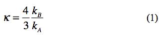
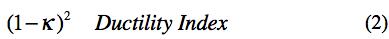
involving the ratio of bond bending to bond stretching stiffness was used to form the ductility index as
The relationship between the nanoscale variable κ and the macroscopic Poisson’s ratio ν was found to be given by
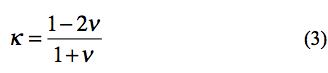
Knowledge of the values of Poisson’s ratios for the (polycrystalline) elements then gave the corresponding ductility indices for the elements, establishing the rank order list of the ductility’s.
The next step leading to the measure of physical ductility is developed here. This is to use the absolute limits on ν of 0 and 1/2 , as derived in Section XII, to require that a relationship between the ductility index (2) and the physical ductility, say D, must have vanishing slopes on a D versus ductility index curve at the limits of the latter, which are 0 and 1. Thinking of this relationship as y = f(x), then an explicit form for it must be found. There is no unique form for this, but the lowest order polynomial to satisfy the end conditions is given by
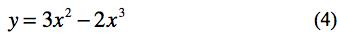
The plot of (4) is shown in Fig. 1.
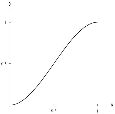
Fig. 1 Equation (4) form
Of necessity there is an inflection point involved with (4) that will later relate to the ductile/brittle transition.
Collecting the governing forms for the physical ductility together, then the nanoscale variable κ is found from experimental values of ν for the elements from (1). Next, the ductility index is formed as
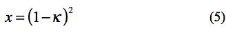
Then the physical ductility, D, is determined by
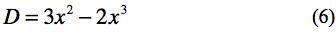
When (5) and (6) are combined it is found that the physical ductility, D, is a sixth degree polynomial in κ. This might at first seem surprising but actually it is consistent with the modeling of atomic potentials that are generally found to be of high order polynomial form.
The final step is to take the table of elements from Section XII to obtain the following table of physical ductility’s for the solids forming elements.
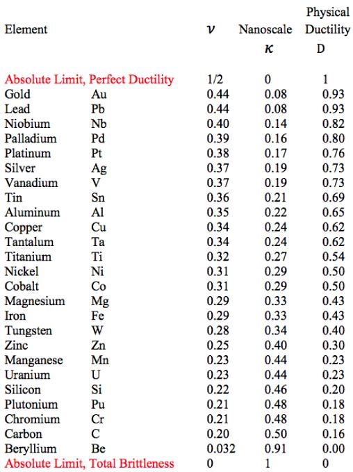
Table 1 Physical Ductility’s
A graph of the physical ductility’s from (6) along with the values for a few of the elements from Table 1 are given in Fig. 2 below.
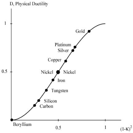
Fig. 2 Physical ductility’s
The double entry of nickel in Fig. 2 will be explained a little later. It must be cautioned that these physical ductility’s for the elements could be considerably different from those for the compounds and alloys of the same generic names. Still, most of those elements in Table 1 are in general agreement with perceived ductility levels. Take iron for example, with its physical ductility of D = 0.43. For the general ductility treatment of Section VII the ductility measure for cast iron is about that of T/C = 2/5 = 0.4, giving general agreement between the two very different methodologies, but which still have the same limits.
Now it will be shown that there is some correlation between the physical ductility’s and the number of shells in each electronic configuration. First, some technical editing will be applied to the list of elements in Table 1. The actinides are in a class by themselves. Accordingly the uranium and plutonium entries in Table 1 will be eliminated from the present considerations. Somewhat related to this, the two elements tantalum and tungsten will also be eliminated in the following list since they are adjacent to the lanthanides and actinides in the Periodic Table. In addition, four slight changes in positions in Table 1 will be taken as follows. The following adjacent elements will be give reversed order of appearance in the list: palladium with platinum, vanadium with tin, aluminum with copper, and finally silicon with chromium These changes are within the experimental errors of the associated Poisson’s ratios: 0.39 versus 0.38, 0.37 versus 0.36, 0.35 versus 0.34, and finally 0.22 versus 0.21, respectively.
With the above slight changes the modified Table 1 will be restated in terms of the electronic configurations while still preserving the rank order list of decreasing ductility’s. The resulting list is shown in Table 2.
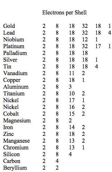
Table 2 Electronic configurations, decreasing ductility’s
It is seen from Table 2 that there is a quite distinct relation between the number of electron shells and the relative ductility levels. In general, but with exceptions, the fewer the number of electron shells, the lower is the degree of ductility. The most ductile elements have 5 or 6 shells, while the least ductile (most brittle) have 2 or 3 shells.
Many interesting comparisons can be made with sub-groups of elements in Table 2. For example, compare the electronic structures of gold, silver, and copper, and their position within Table 2. All are from the 11th group in the Periodic Table. The comparison of aluminum, magnesium, and silicon is interesting and significant.
The element nickel is particularly interesting. As seen from Table 1 and Fig. 1 nickel is right at the ductile/brittle transition. In addition to its electronic configuration of 2, 8, 17, 1 shown in Table 2 it has another stable configuration of 2, 8, 16, 2 that gives virtually the same properties. Nickel is the only element in Tables 1 and 2 that admits the dual electronic configurations. One might speculate that nickel’s 2, 8, 17, 1 configuration leans slightly toward the ductile side because of its coordination with the 2, 8, 18, 1 configuration of copper. Conversely, nickel’s 2, 8, 16,2 configuration might shade slightly toward the brittle side because of its coordination with the 2, 8, 15, 2 configuration of cobalt and the 2, 8, 14, 2 configuration of iron. All four elements are consecutive entries in the 4th period of the Periodic Table.
Using the numbers of shells for the elements in Table 2 along with the physical ductility values in Table 1, the following list of average physical ductility’s versus the number of shells is found to be given by
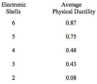
Table 3 Average ductility’s for Table 2 elements
As seen from Table 2 there is a broad range of 4 shell elements that nevertheless have widely varying ductility’s. Obviously many other electron level effects also contribute to the level of ductility for any given element.
Although one could go further this direction and correlate ductility levels with the types of orbitals, it would not seem to be an enlightening direction. Since all of this follows form the differentiation of the nanoscale bond bending and bond stretching mechanisms there could be a considerable opportunity to examine these effects directly by using density functional theory.
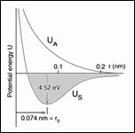
The final thing to be considered here is the ideal, theoretical strength of the solids forming elements. To begin, it is much easier to estimate the ideal strain to failure of the elements than it is the ideal stress to failure. This is because nondimensional strain to failure can be interpreted directly at the atomic level, as follows. For a given element that has N electronic shells, take the spacing between the shells as being unity and uniform between shells. The outermost Nth shell in the deformed configuration under load has its electrons as moving toward a hypothetical N+1 shell. If they were to succeed in moving to the N+1 shell it would be transmuted into a new element. But that is not possible and instead failure is taken to occur at the extreme bond stretching position. Failure is explicitly taken to occur when the outermost electron shell is deformed to a position mid-way between the undeformed position of the outermost Nth shell and that of the hypothetical N+1 shell. The strain that occurs at this extreme deformed position of failure is then
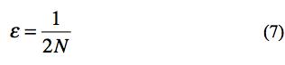
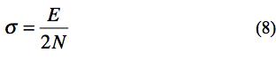
To form the theoretical strength, the macroscopic modulus of elasticity is combined with (7) to give the ideal, theoretical strength as
Using examples from 6, 4, and 2 shell elements gives their theoretical strengths as
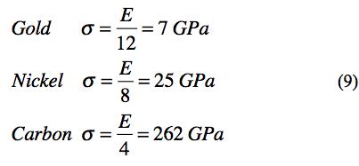
These are comparable to the widely quoted ideal strength of about σ = E/10, Kelly [1], Cottrell [2]. The present estimates based upon atomic structure puts a little sharper definition on the theoretical strength.
These ideal strengths are many orders of magnitude larger than the observable and realistic strengths. This shows the extraordinary power of flaws and defect structures to control and dictate the usable strengths.
In the three dimensional solids forming elements and materials made from the elements it is not possible to have a defect free isotropic arrangement of the atoms. All arrangements of atoms involve crystal structures in randomly oriented polycrystalline grains to give isotropy. In addition, there may be dislocations, vacancies and other imperfections in each individual crystal grain. At a little larger scale, all grain boundaries between individual crystals represent defect structures. The ideal, theoretical strength ignores these realities. Nevertheless it is still interesting as representing the ultimate potential performance level and also helpful in comparisons, as (9) shows.
Graphene is the only perfect, isotropic form of the elements, but it is of a two dimensional not three dimensional arrangement of the atoms. It is interesting to observe that the strain at failure for graphene is observed by Lee et al [3] from nanoscale indentation experiments to be 25%, which is the same as that predicted by (7) for the two shell carbon atom. However, it must be kept in mind that there can be and is a need for damage tolerant materials. The role of dislocations in gold is a good example. The ideal strength property for gold is completely irrelevant. The incredible ductility/plastic flow capability of gold is one of its prime mechanical assets.
References
1. Kelly, A. and Macmillan, N. H. (1987), Strong Solids, Oxford Univ. Press, Oxford.
2. Cottrell, A. H. (1981), The Mechanical Properties of Matter, Krieger, Malabar, FL.
3. Lee, C., Wei, X., Kysar, J. W., and Hone, J. (2008), “Measurement of the Elastic Properties and Intrinsic Strength of Monolayer Graphene”, Science 321, 385-388.
Oct. 21 2012